Confidence Interval for µ

STAT 218 - Week 4, Lecture 3

What Did We Learn This Week?

On Monday, we explored a method for estimating a confidence interval for a long-run proportion or population proportion.
- We found the confidence interval by conducting repeated tests of significance and changing the probability specified by the null hypothesis to see whether or not the hypothesized value was plausible.
Yesterday, we explored that there are also other ways to approximate a confidence interval.
- “Two standard deviation method” (or 2SD method)
  - The idea of standardization to construct confidence intervals which gives us an approximate 95% confidence interval.
  - typically based on simulation
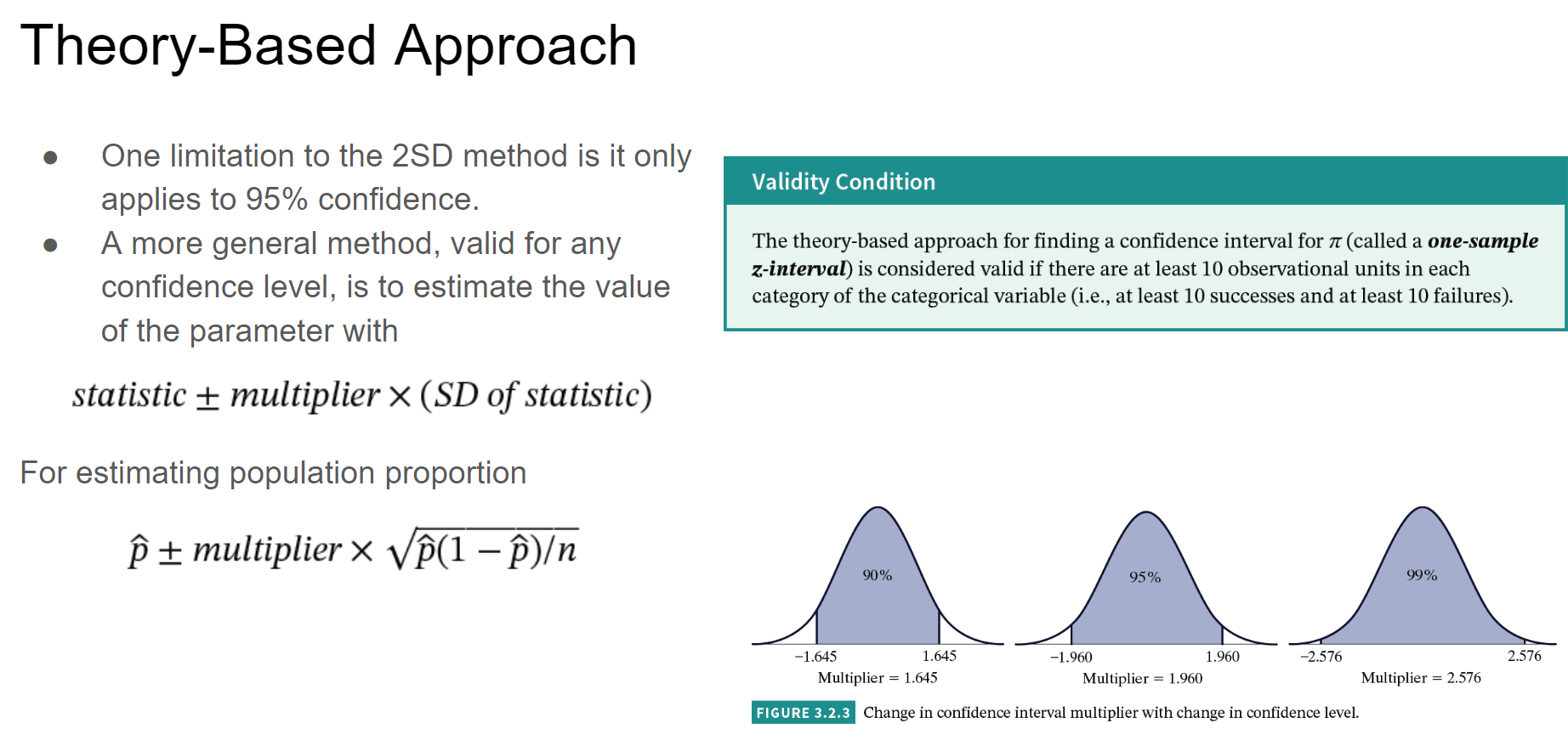
Theory-based approach to generating confidence intervals,
- avoids the need to use simulation altogether.
allows us to easily use any confidence level we would like, not just 95%.

# CI Methods for a Single Mean

Introduction

In previous chapters, we were focusing on inferences about a population proportion (categorical variable).
Now, we will focus on data consisting of a single quantitative variable.
We will make inferences about a population mean by creating confidence intervals.
- 2SD approach
- Theory-based approach
  - The probability distribution in this section is called the t-distribution

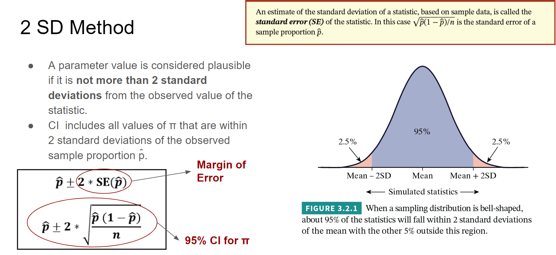
2 SD Confidence Interval Method for a Single Mean

2 SD approach should be reasonable as long as the sampling distribution of the sample means is reasonably symmetric.
- Previously, when we didn’t know σ (the population standard deviation), we learnt that we could approximate σ/√n with s/√ n.
- We also saw that an estimate of the standard deviation of a statistic is often referred to as the standard error.

The general form of a confidence interval is

\[ \\ statistic \pm multiplier \times (SD \ of \ statistic) \]

Here, our statistic will be the sample mean and multiplier will be 2.

\[ \\ \bar{x} \pm 2 \times (s/ \sqrt{n}) \]

Theory-Based Confidence Interval for a Single Mean

Important Symbols

To distinguish a quantitative variable from a categorical variable, we use different symbols to show population parameters and sample statistics.

Parameters

\(\mu\) = population mean

\(\sigma\) = population standard deviation

Statistics

\(\bar{x}\) = sample mean

\(s\) = sample standard deviation

Student’s t distribution

What is t distribution?

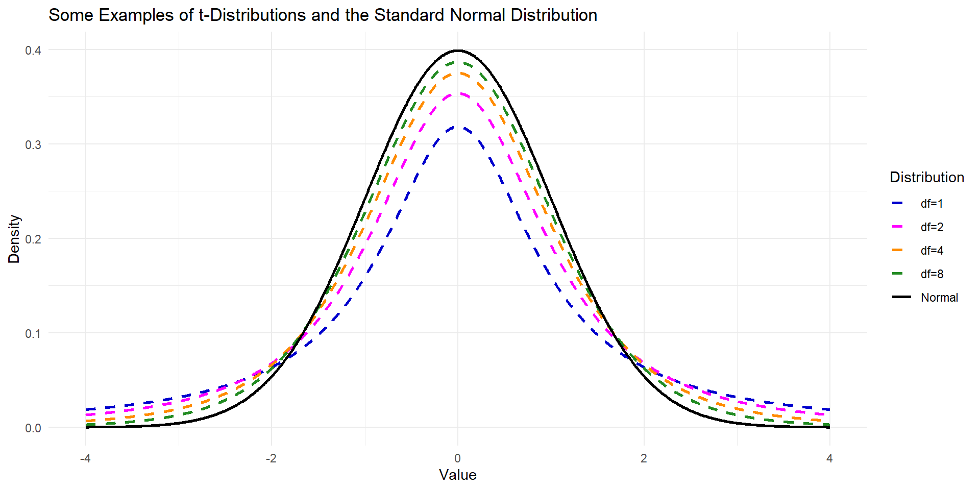
\(t\)-distribution is another bell shape and symmetric distribution that can be useful if we do not know anything about population parameters.
The \(t\)-distribution is always centered at zero and has a single parameter: degrees of freedom.
- The shape of the distribution depends on the degrees of freedom.
Broadly speaking, we use \(t\)-distribution with \(df = n − 1\)
- to model the sample mean when the sample size is \(n\).
- As the \(df\) is increasing, the \(t\)-distribution will look more like the standard normal distribution
  - when the \(df\) is about 30 or more, the \(t\) -distribution is nearly indistinguishable from the normal distribution.

What is t distribution?

Comparison of t and the Standard Normal Distribution

Both are symmetric and bell-shaped but \(t\)-distribution has a larger standard deviation.
The \(t\)-distribution has a single parameter: degrees of freedom.
Standard Normal Distribution has two parameters: \(\mu\) and \(\sigma\).

Statistical Estimation

Statistical estimation is a form of statistical inference in which we use the data to
1. determine an estimate of some feature of the population and
2. assess the precision of the estimate.

An Example for Statistical Estimation

Let’s have a look wing areas of 14 male Monarch butterflies at Oceano Dunes State Park in California

\(\bar{x} = 32.81\) \(cm^2\) and \(s= 2.48\) \(cm^2\)

Suppose we consider these 14 observations as a random sample from a population.

\(\mu\) = the (population) mean wing area of male Monarch butterflies in the Oceano Dunes region
\(\sigma\) = the (population) SD of wing area of male Monarch butterflies in the Oceano Dunes region

From the sample data we have, we can say that

32.81 is an estimate of \(\mu\).
2.48 is an estimate of \(\sigma\).

Statistical Estimation cont.d

We should be aware of the fact that these estimates are subject to sampling error.

Warning

This is NOT measurement error;
- No matter how accurately each individual butterfly was measured, the sample information is imperfect
  - due to the fact that only 14 butterflies were measured, rather than the entire population of butterflies.

Broadly speaking, for a sample of observations on a quantitative variable X
- \(\bar{x}\) is an estimate of \(\mu\).
- s is an estimate of \(\sigma\).

And our goal is to estimate \(\mu\).

Confidence Interval

An Introduction to Confidence Interval - I

Our aim is to…
- determine an estimate of \(\mu\)
  - \(\bar{x}\) was an estimate of \(\mu\)
We also know that the difference between \(\bar{x}\) and \(\mu\) is rarely more than a few standard errors.

Tip

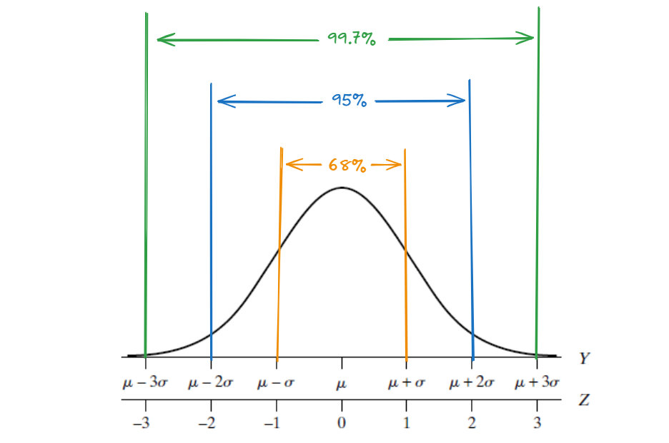
If \(Z\) is a standard normal random variable, then the probability that \(Z\) is between \(\pm\) 2 is about 0.95 (OR 95% if we remember The 68/95/99.7 rule)

An Introduction to Confidence Interval - II

To understand how to calculate confidence intervals, we need to have

standardization formula
standard error
multiplier (will be given) and
solve an equation that composed of these

Standard Error of the Mean

Standar error is the standard deviation of the null distribution.
The standard error of the mean is calculated as follow:

\[ SE_\bar{X} = \frac{s}{\sqrt{n}} \]

Monarch Butterfly Revisited - I

Let’s have a look wing areas of 14 male Monarch butterflies at Oceano Dunes State Park in California

\(\bar{x} = 32.8143 \ cm^2\) and \(s= 2.4757 \ cm^2\)

Suppose we consider these 14 observations as a random sample from a population. For the multiplier, it is given as

\[ \\ multiplier = 2.160 \]

95% confidence interval (CI) for \(\mu\) can be calculated as following:

\(\bar{x} = 32.8143 \ cm^2\) and \(s= 2.4757 \ cm^2\)

\[ \\95 \% \ CI = (\bar{x} \pm multiplier \ \times \ SE_{\bar{x}}) \\95 \% \ CI = (32.8143 \pm 2.160 \ \times \ 2.4757 / \sqrt{14}) \]

\[ \\= 32.81 \pm 1.43 \\ 31.43 \ cm^2 < \mu < 34.2 \ cm^2 \\ OR \\ 95 \% \ CI = (31.43,34.2) \]

Monarch Butterfly Revisited - II

90% confidence interval (CI) for \(\mu\) can be calculated as following (multiplier:1.771):

\(\bar{x} = 32.8143 \ cm^2\) and \(s= 2.4757 \ cm^2\)

\[ \\90 \% \ CI = (\bar{y} \pm multiplier \ \times SE_{\bar{x}}) \\90 \% \ CI = (32.8143 \pm 1.771 \ \times \ 2.4757 / \sqrt{14}) \]

\[ \\= 32.81 \pm 1.17 \\ 31.64 \ cm^2 < \mu < 33.98 \ cm^2 \]

What is the difference between 90% CI and 95% CI?

Why are we 95% confident?

Understanding Confidence Intervals

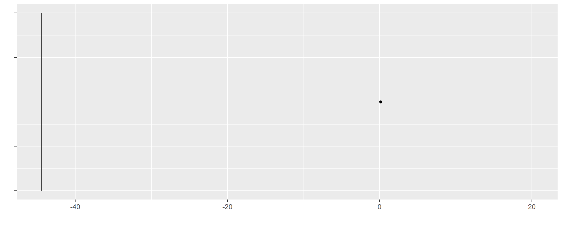
To help you visualize, imagine we have a population, and from that population, we randomly select a group of 20 observational units

95%CI = (-44.47, 20.13)

Understanding Confidence Intervals

If we repeat this process 100 times, creating 100 different samples of 20 observational units each, we would end up with 100 different samples drawn from the population.

Understanding Confidence Intervals

If we calculate confidence intervals for each of these 100 samples, we will find that…

Around 95% of these intervals capture the true population mean
We are 95% confident that the true population mean is in this confidence interval.

Confidence Interval - Verbal Explanation

And…

If we calculate confidence intervals for each of these 100 samples, we will find that around 95% of these intervals capture the true population mean.
We are 95% confident that the true population mean is in this confidence interval.

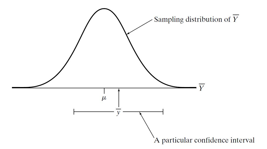
Confidence Interval and Sampling Distribution

Planning a Study to Estimate μ

Before collecting data for a research study, it is wise to consider in advance whether the estimates generated from the data will be sufficiently precise.
- It can be painful indeed to discover after a long and expensive study that the standard errors are so large that the primary questions addressed by the study cannot be answered.
The precision with which a population mean can be estimated is determined by two factors:

the population variability of the observed variable Y, and
the sample size.

Planning a Study to Estimate μ

In some situations the variability of Y cannot, and perhaps should not, be reduced.
- For example, a wildlife ecologist may wish to conduct a field study of a natural population of fish; the heterogeneity of the population is not controllable and in fact is a proper subject of investigation.
On the other hand, it is often appropriate, especially in comparative studies, to reduce the variability of Y by holding extraneous conditions as constant as possible.
- For example, physiological measurements may be taken at a fixed time of day; tissue may be held at a controlled temperature; all animals used in an experiment may be the same age

What sample size will be needed?

Recall that

\[ SE_{\bar{x}} = \frac{s}{\sqrt{n}} \]

We can use this formula to determine our sample size as follows:

\[ Desired \ SE = \frac{Guessed \ SD}{\sqrt{n}} \]

Same Example from Last Week - IV

Suppose the researcher is now planning a new study of butterflies Monarch butterflies at Oceano Dunes State Park in California and has decided that it would be desirable that the SE be no more than \(0.4 \ cm^2\)

\(\bar{y} = 32.8143 \ cm^2\) and \(s= 2.4757 \ cm^2\)

\[ SE_{\bar{y}} = s / \sqrt{n} \]

\[ Desired \ SE = Guessed \ SD / \sqrt{n} \]

\[ \\Desired \ SE = 2.48 / \sqrt{n} \ \le 0.4 \\ n\ge 38.4 \] \[ \\ at \ least \ 39 \ butterflies \]

You may wonder how a researcher would arrive at a value such as \(0.4 \ cm^2\) for the desired SE. Such a value is determined by considering how much error one is willing to tolerate in the estimate of μ.