[1] 37One Way ANOVA
Week 9, Lecture 4 Lab 6
Before Proceeding Further…
Let me introduce you the pipe operator ( |> )
Shortcut: Ctrl (Command) + Shift + M
Combine 35, 30, and 45 and then
Take the mean and then
Round the output
Like a composite function such as (\(f\circ g\circ h(x)\))
One Way ANOVA
Research Question and Data Set
The Wolf River in Tennessee flows past an abandoned site once used by the pesticide industry for dumping wastes, including chlordane (pesticide), aldrin, and dieldrin (both insecticides). These highly toxic organic compounds can cause various cancers and birth defects. As these compounds are denser than water and their molecules tend to stick to particles of sediment, they are more likely to be found in higher concentrations near the bottom.
Now we are collecting a total of 30 random samples from this river to test if there is a difference between the mean aldrin concentrations among the three levels (surface, middepth, bottom)? (Set the alpha value as 0.05 for this study.)
Step 3. Checking Conditions/Assumptions:
Assumptions/Conditions
1. The observations should be independent within and between groups
- If the data are a simple random sample from less than 10% of the population, this condition is satisfied
- Carefully consider whether the data may be independent (e.g. no pairing)
- Always important, but sometimes difficult to check
2. The observations within each group should be nearly normal
- Normality can be roughly checked by making a histogram and normal quantile plot of the data if your sample size is large.
- If your sample size is small, you should use
shapiro.test()for each group in your categorical variable.
3. The variability across the groups should be about equal
- Especially important when the sample sizes differ between groups.
- The condition of normal populations with equal standard deviations is less crucial if the sample sizes (\(n_i\)) are large and approximately equal.
- As a rule of thumb, we would like the largest sample SD divided by the smallest sample SD to be less than 2 or so.
- If this ratio is much larger than 2, then we cannot be confident in the P-value from the ANOVA, particularly if the sample sizes are small and unequal.
Failing to check conditions may affect the test’s error rates.
Step 3. Checking Conditions/Assumptions - Normality
Step 3. Checking Conditions/Assumptions - Homogeneity of Variance
# A tibble: 3 × 3
  depth     mean    sd
  <chr>    <dbl> <dbl>
1 bottom    6.04 1.58
2 middepth  5.05 1.10
3 surface   4.2  0.660
Let’s check if the largest sample SD divided by the smallest sample SD to be less than 2
Step 4. Calculate F statistic and find the p-value
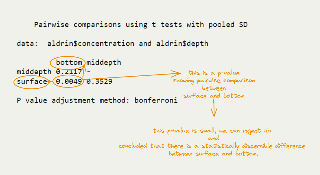
Post Hoc
A significant F-test indicates that we can reject null hypothesis, which states that population means are equal.
- However, it does not tell us which of the groups differ.
- We need to conduct post-hoc tests. Post-hoc tests are designed to help protect against the likelihood of Type-I error.
How to Evaluate This Output?
