Correlation & Least Squares Regression

Week 9, Lecture 3 Lab 7

December 3^th, 2024

Correlation

Let’s Load This Week’s Data Set

library(openintro)
library(tidyverse)
data("babies")
glimpse(babies)

Rows: 1,236
Columns: 8
$ case      <int> 1, 2, 3, 4, 5, 6, 7, 8, 9, 10, 11, 12, 13, 14, 15, 16, 17, 1…
$ bwt       <int> 120, 113, 128, 123, 108, 136, 138, 132, 120, 143, 140, 144, …
$ gestation <int> 284, 282, 279, NA, 282, 286, 244, 245, 289, 299, 351, 282, 2…
$ parity    <int> 0, 0, 0, 0, 0, 0, 0, 0, 0, 0, 0, 0, 0, 0, 0, 0, 0, 0, 0, 0, …
$ age       <int> 27, 33, 28, 36, 23, 25, 33, 23, 25, 30, 27, 32, 23, 36, 30, …
$ height    <int> 62, 64, 64, 69, 67, 62, 62, 65, 62, 66, 68, 64, 63, 61, 63, …
$ weight    <int> 100, 135, 115, 190, 125, 93, 178, 140, 125, 136, 120, 124, 1…
$ smoke     <int> 0, 0, 1, 0, 1, 0, 0, 0, 0, 1, 0, 1, 1, 1, 0, 0, 1, 1, 0, 1, …

Correlation Coefficient

The correlation coefficient is rarely computed by hand so we will use the cor() function to obtain our observed sample correlation coefficient.

cor(babies$gestation, babies$bwt, use = "na.or.complete")

[1] 0.407854

Direction of the relationship: Positive Relationship

Outliers

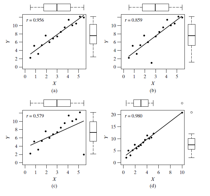
Outliers can distort regression analysis in two ways:

1. by inflating \(s_e\) and reducing correlation; and
2. by unduly influencing the regression line.

Outliers

• Leverage points are points that have the potential to greatly influence the slope of the fitted regression model.
  • The further a point’s X value is from the center of the X distribution, the more leverage that point has on the overall regression model.
• Plots (c) and (d) display examples of leverage points.
  • In plot (c) the leverage point is shown to actually exert its leverage on the line, tipping the regression from the bulk of the data.
• A point that has a large effect on the regression model is called an influential point.
  • Plot (d) shows a leverage point (because of the extreme X value) that is not influential because the regression line does not get pulled away from the trend in the bulk of the data.
• Note that the outlier in plot (b) is not considered a leverage point—its ability to affect the slope of the line is weak as its X value is near the center of the X distribution.

Scatterplot

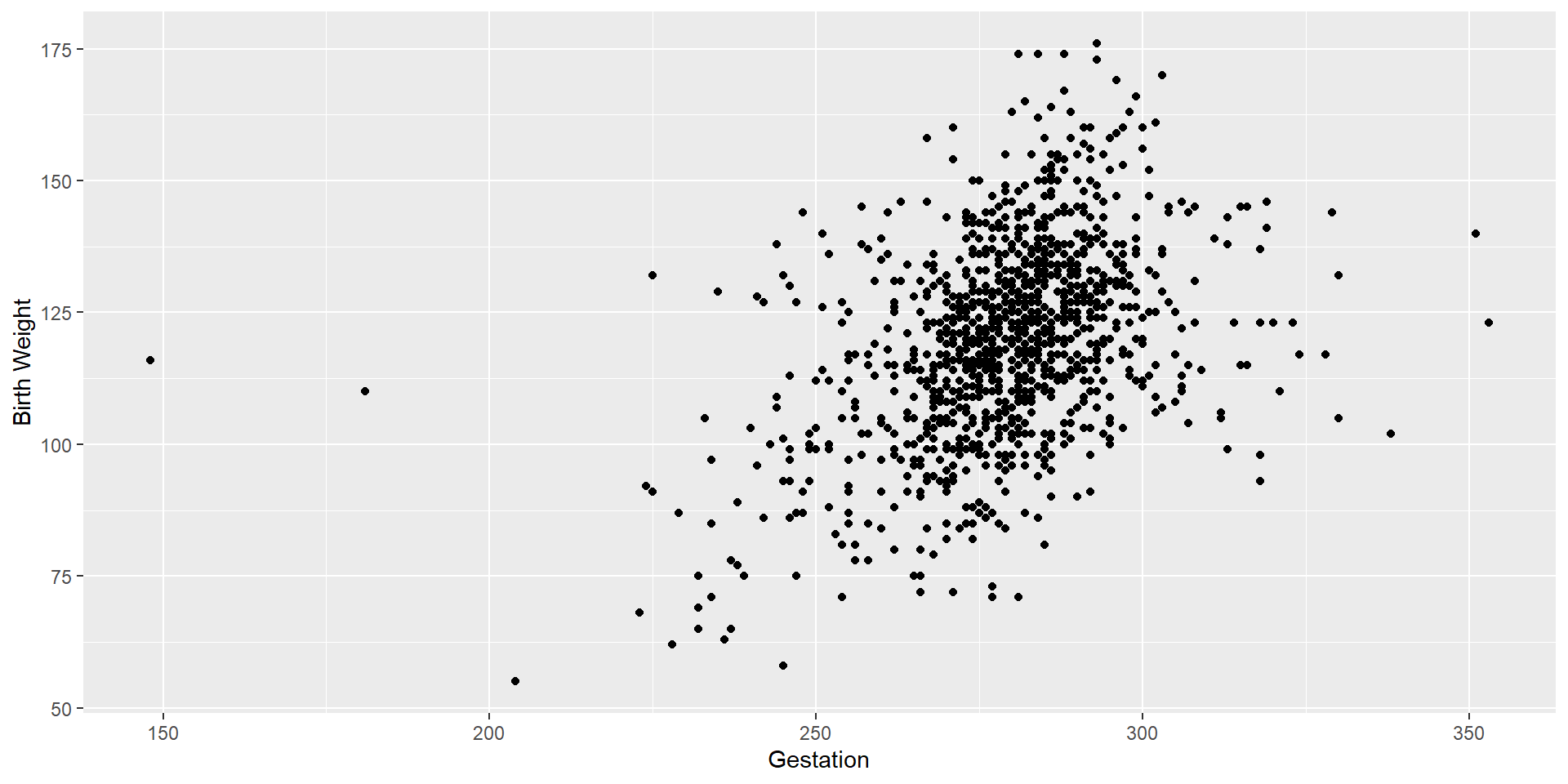
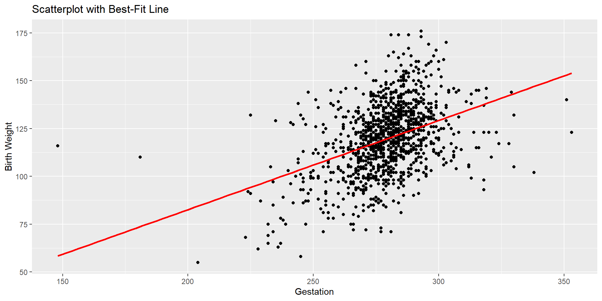
Let’s see the scatterplot to look for potential outliers.

ggplot(na.omit(babies), aes(x = gestation, y = bwt)) +
  geom_point() +
  labs(x = "Gestation", y = "Birth Weight")

Scatterplot

Let’s see the scatterplot to look for potential outliers.

Let’s clean the data set

We see two outliers on the left-hand side of the scatterplot. Let’s remove those outliers.

babies1 <- babies %>%
  filter(case != 261 & case != 870 & case !=979) 
# this removes three outliers whose case numbers are 261, 870 & 979

Check your environment pane and notice that the number of observations is decreased.

Let’s see the changes

Let’s check the correlation coefficient and scatterplot again.

cor(babies1$gestation, babies1$bwt, use = "na.or.complete")

[1] 0.4144271

ggplot(na.omit(babies1), aes(x = gestation, y = bwt)) +
  geom_point() +
  labs(x = "Gestation", y = "Birth Weight")

Let’s see the changes

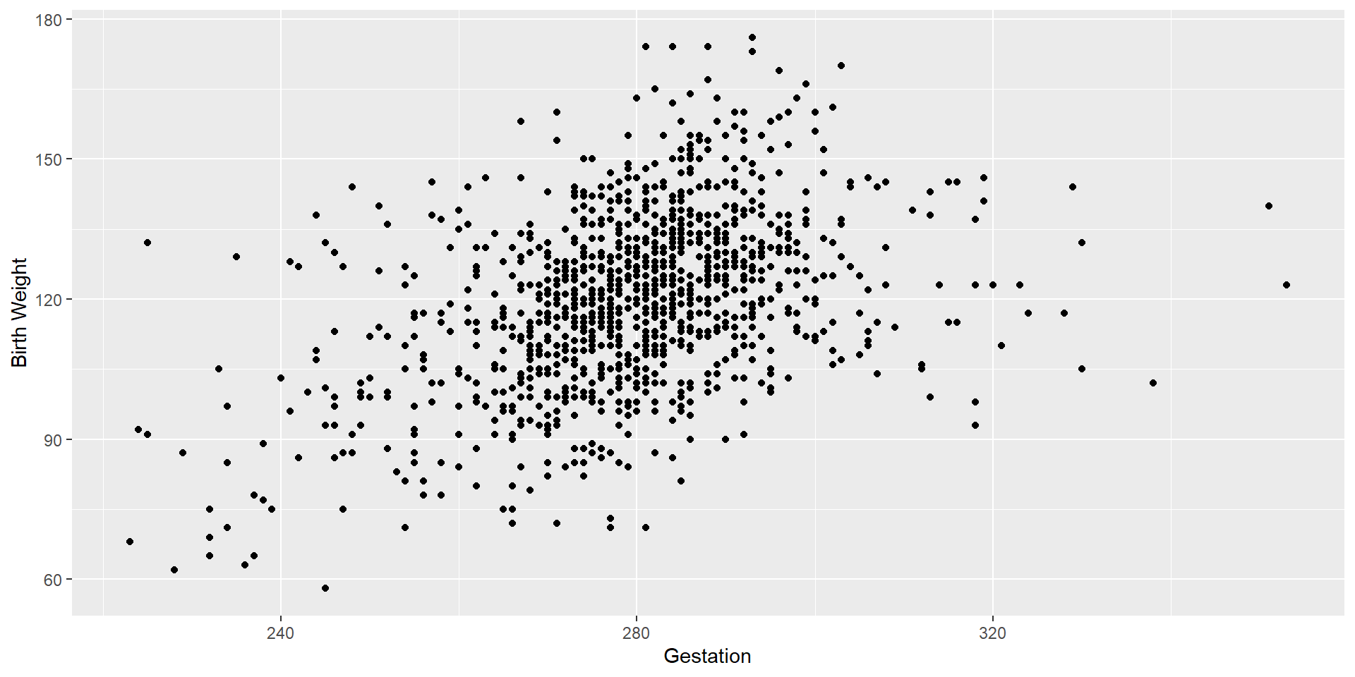
We see some potential outliers on the right-hand side of the scatterplot. Let’s remove those as well.

Let’s clean the data set one more time

babies2 <- babies1 %>%
  filter(case != 1173 & case != 11 & case != 1200 & case != 153 & case != 762 & case != 970 & case != 241 & case != 254  & case != 1003 & case != 461  & case != 1045 & case != 1220)

Let’s see the changes

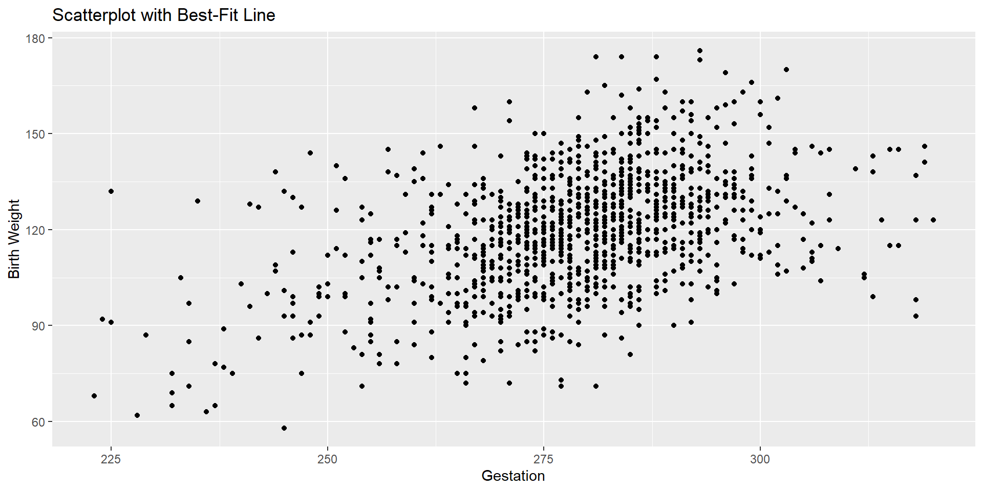
Let’s check one last time and decide if we really need to remove outliers.

cor(babies2$gestation, babies2$bwt, use = "na.or.complete")

[1] 0.4387897

ggplot(na.omit(babies2), aes(x = gestation, y = bwt)) +
  geom_point() +
  labs(x = "Gestation", y = "Birth Weight")

Let’s see the changes

Let’s Brainstorm Together!

• Leverage points vs influential points
• Compare those correlation coefficients that we calculated
• Do we need to delete those outliers?

Bivariate Regression

Research Question and Data Set

Understanding Birth Weight and Gestation: A Least Squares Regression Analysis

In the area of prenatal care and childbirth, understanding the relationship between gestation period and birth weight is crucial. We often speculate about how the duration of pregnancy might be related with the weight of a newborn.

In the babies dataset, each observation includes information about gestation period and birth weight. We want to investigate if there’s a linear relationship between these two variables.

Hypothesis Testing

We will test the null hypothesis

\[ H_0: \beta_1 = 0 \] against the non-directional alternative

\[ H_A: \beta_1 \neq 0 \] Verbal Hypotheses are as follows:

\(H_0\): Birth weight is not linearly related to gestation

\(H_A\): Birth weight is linearly related to gestation

Important

Note that the test on \(\beta_1\) asks whether, assuming that the linear model holds, we can conclude that the slope is nonzero.

Checking Conditions/Assumptions:

Assumptions/Conditions

1. The observations should be independent

2. Linearity

• The relationship between the explanatory and the response variable should be linear.
  • Check either using (1) a scatterplot of the data, or (2) a residuals plot.

3. The residuals should be nearly normal.

• This condition may not be satisfied when there are unusual observations that don’t follow the trend of the rest of the data.

• Check using (1) a histogram or (2) normal probability plot of residuals.

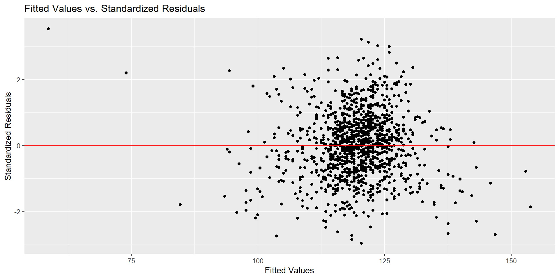
4. Constant Variability - Homoscedasticity

• The variability of points around the least squares line should be roughly constant.

• This implies that the variability of residuals around the 0 line should be roughly constant as well.

• Check using (1) a histogram or (2) normal probability plot of residuals.

Before Checking the Conditions

Step 2: Generate Your Model

IMPORTANT: The codes I use include the babies dataset. If you chose a different dataset, such as babies1 or babies2(see your environment pane), be sure to replace babies with the correct dataset name in all instances.

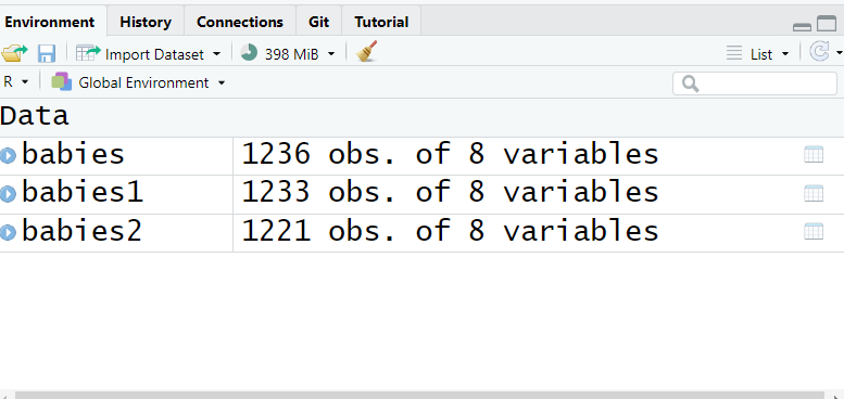
Before Checking the Conditions

• In bivariate regression, we need to first model the relationship and check the conditions after because we need residuals.

# I am using the babies dataset because I decided not to delete outliers
fit <- lm(babies$bwt ~ babies$gestation)
summary(fit)

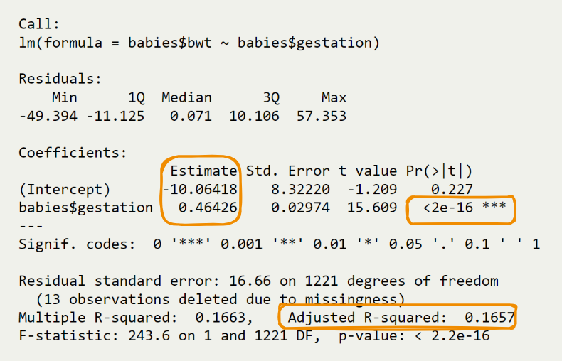
Call:
lm(formula = babies$bwt ~ babies$gestation)

Residuals:
    Min      1Q  Median      3Q     Max 
-49.394 -11.125   0.071  10.106  57.353 

Coefficients:
                  Estimate Std. Error t value Pr(>|t|)    
(Intercept)      -10.06418    8.32220  -1.209    0.227    
babies$gestation   0.46426    0.02974  15.609   <2e-16 ***
---
Signif. codes:  0 '***' 0.001 '**' 0.01 '*' 0.05 '.' 0.1 ' ' 1

Residual standard error: 16.66 on 1221 degrees of freedom
  (13 observations deleted due to missingness)
Multiple R-squared:  0.1663,    Adjusted R-squared:  0.1657 
F-statistic: 243.6 on 1 and 1221 DF,  p-value: < 2.2e-16

• We employ the lm function in R to perform a bivariate regression analysis.

• The formula lm(babies$bwt ~ babies$gestation) indicates that we are modeling birth weight (bwt) as a linear function of gestation period (gestation).

  • The subsequent summary(fit) provides detailed statistics about the regression model.

Checking Conditions- Linearity with Scatterplot

ggplot(na.omit(babies), aes(x = gestation, y = bwt)) +
  geom_point() +
  geom_smooth(method = "lm", se = FALSE, color = "red") +
  labs(title = "Scatterplot with Best-Fit Line",
       x = "Gestation",
       y = "Birth Weight")

Checking Conditions - Linearity with Residuals Plot

# get list of residuals  
res <- resid(fit) 
res.stdres <- rstandard(fit) # standardized residuals

# produce residual vs. fitted plot 
ggplot(data.frame(fitted = fitted(fit), stdres = res.stdres), 
       aes(x = fitted, y = stdres)) +
  geom_point() +
  geom_hline(yintercept = 0, linetype = "solid", color = "red") +
  labs(title = "Fitted Values vs. Standardized Residuals",
       x = "Fitted Values",
       y = "Standardized Residuals") +
  theme_minimal()

Checking Conditions - Linearity with Residuals Plot

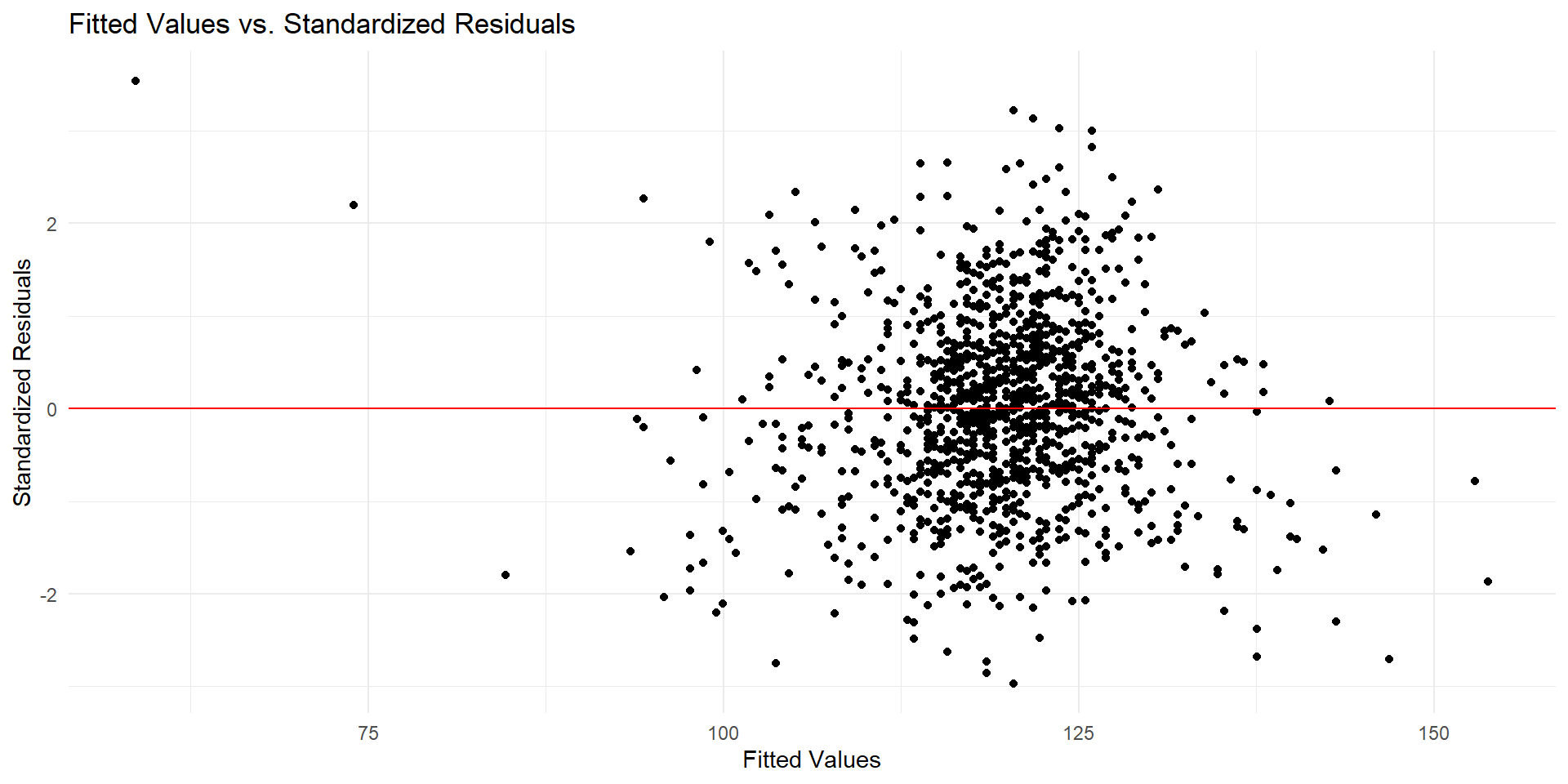
Checking Conditions - Normality

# create Q-Q plot for residuals 
qqnorm(res.stdres) # by using standardized residuals
  
# add a straight diagonal line to the plot 
qqline(res.stdres)

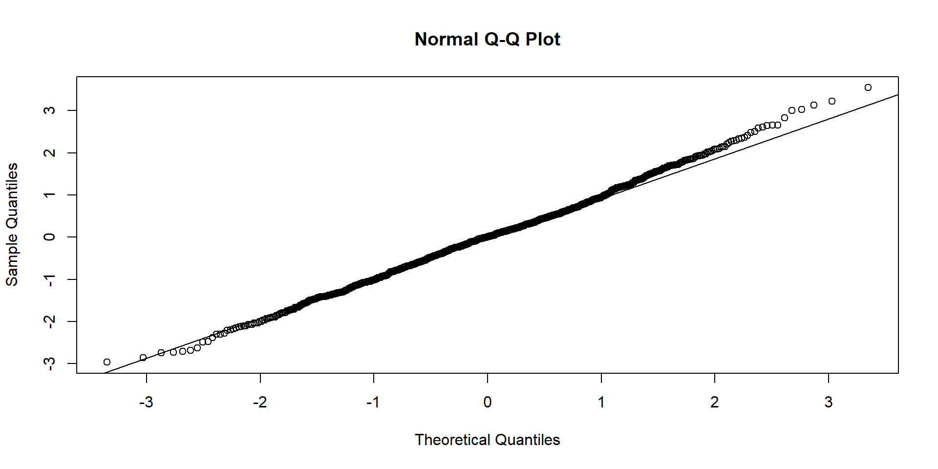
Checking Conditions - Homoscedasticity

# get list of residuals  
res <- resid(fit) 
res.stdres <- rstandard(fit) # standardized residuals

# produce residual vs. fitted plot 
ggplot(data.frame(fitted = fitted(fit), stdres = res.stdres), 
       aes(x = fitted, y = stdres)) +
  geom_point() +
  geom_hline(yintercept = 0, linetype = "solid", color = "red") +  # Add a horizontal line at 0
  labs(title = "Fitted Values vs. Standardized Residuals",
       x = "Fitted Values",
       y = "Standardized Residuals")

Checking Conditions - Homoscedasticity

Draw Conclusion

Draw Conclusion

Call:
lm(formula = babies$bwt ~ babies$gestation)

Residuals:
    Min      1Q  Median      3Q     Max 
-49.394 -11.125   0.071  10.106  57.353 

Coefficients:
                  Estimate Std. Error t value Pr(>|t|)    
(Intercept)      -10.06418    8.32220  -1.209    0.227    
babies$gestation   0.46426    0.02974  15.609   <2e-16 ***
---
Signif. codes:  0 '***' 0.001 '**' 0.01 '*' 0.05 '.' 0.1 ' ' 1

Residual standard error: 16.66 on 1221 degrees of freedom
  (13 observations deleted due to missingness)
Multiple R-squared:  0.1663,    Adjusted R-squared:  0.1657 
F-statistic: 243.6 on 1 and 1221 DF,  p-value: < 2.2e-16

The regression equation is___________________

\[ \hat{y} = b_0 + b_1X \]